
Build a Traffic Sign Recognition Project
The goals / steps of this project are the following:
- Load the data set (see below for links to the project data set)
- Explore, summarize and visualize the data set
- Design, train and test a model architecture
- Use the model to make predictions on new images
- Analyze the softmax probabilities of the new images
- Summarize the results with a written report
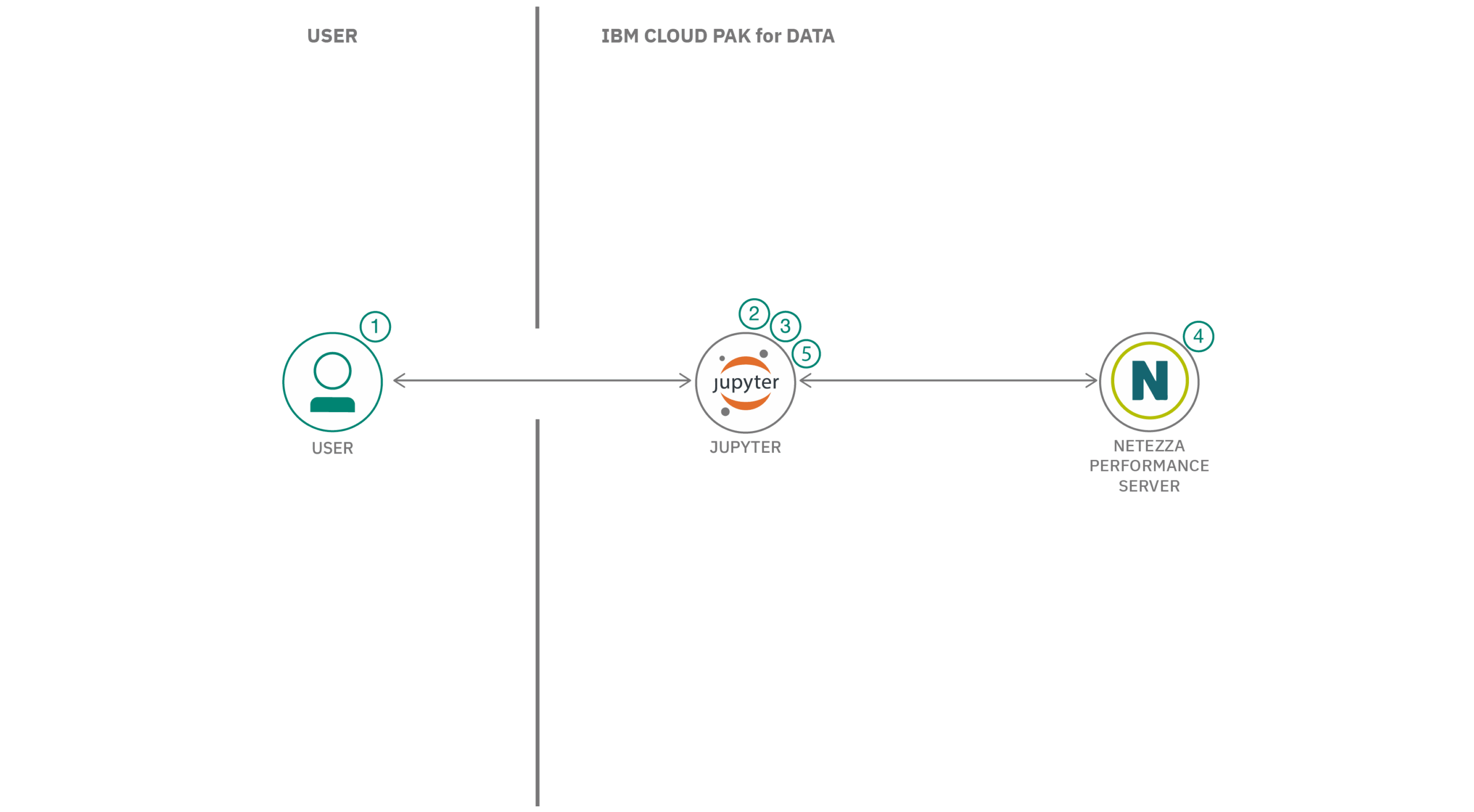
1. Provide a basic summary of the data set and identify where in your code the summary was done. In the code, the analysis should be done using python, numpy and/or pandas methods rather than hardcoding results manually.
I use pickle to import the data into ipython notebook. Then I use numpy to calculate the statistics of the data set.
  import numpy as np

  # Number of training examples
  n_train = len(X_train)

  # Number of testing examples.
  n_test = len(X_test)

  # the shape of an traffic sign image
  image_shape = X_train[0].shape

  # number of unique classes/labels there are in the dataset.
  n_classes = len(np.unique(y_train))

  print("Number of training examples =", n_train)
  print("Number of testing examples =", n_test)
  print("Image data shape =", image_shape)
print("Number of classes =", n_classes)- Image data shape = (32, 32, 3)
- Number of classes = 43
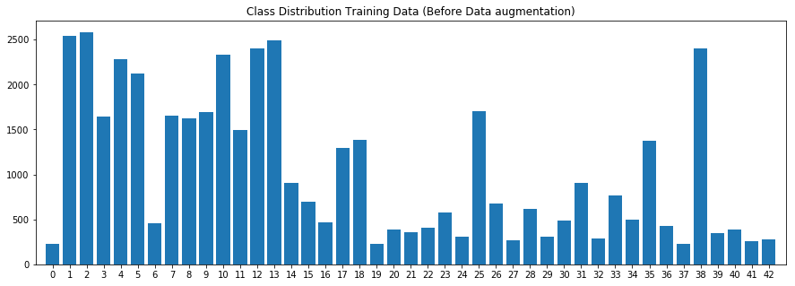
Include an exploratory visualization of the dataset and identify where the code is in your code file.
The chart below is the label distribution, which can show the label distribution are not even, some class have more data then others.

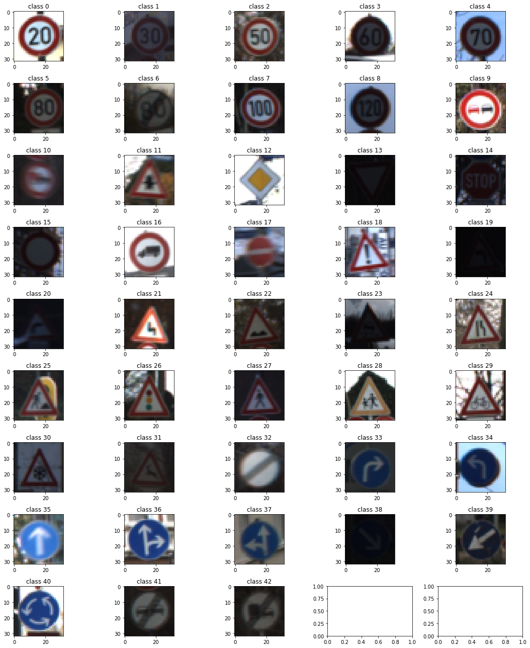
The img below is the chart to show one iamge from each class. Some of them are really dark, which makes difficulties hgiher.

import matplotlib.pyplot as plt
# Visualizations will be shown in the notebook.
%matplotlib inline
#edit matplot size in notebook
plt.rcParams["figure.figsize"] = [15,18]


fig = plt.figure(figsize=(5,5))
f, axarr = plt.subplots(9, 5)
# make it as a sigle dim. array
plts = np.reshape(axarr, -1)

#display one sample from all class
for classId in np.unique(y_train):
    thePicIndex = np.where(y_train == classId)[0]
    myplt = plts[classId]
    myplt.imshow(X_train[thePicIndex[25]])
    myplt.set_title("class " + str(classId))

plt.tight_layout()####1. Describe how, and identify where in your code, you preprocessed the image data. What tecniques were chosen and why did you choose these techniques? Consider including images showing the output of each preprocessing technique. Pre-processing refers to techniques such as converting to grayscale, normalization, etc.
I have few ways to Preprocessed the data set:
- Turn raw images into gray Scale
- Normalize the image to range(0, 1)
- Augmente the images
The advantage of normalizing image is to make gradient descent converge faster.
Gray scale image can reduce the image size, which helps to train the model easier. Image normalized in to range (0, 1) can help model to learn data set. Since the size of dataset not large enough, augmentation on image is necessary.
The Pre-processing params.
- ANGLE_ROTATE = 25
- TRANSLATION = 0.2
- NB_NEW_IMAGES = 10000
def toGrayscale(rgb):
result = np.zeros((len(rgb), 32, 32,1))
result[...,0] = np.dot(rgb[...,:3], [0.299, 0.587, 0.114])
return result
# normalize the images
def normalizeGrascale(grayScaleImages):
return grayScaleImages/255
def processImages(rgbImages):
return np.array(normalizeGrascale(toGrayscale(rgbImages)))
def transformOnHot(nbClass, listClass):
oneHot = np.zeros((len(listClass), nbClass))
oneHot[np.arange(len(listClass)), listClass] = 1
return np.array(oneHot)
def augmenteImage(image, angle, translation):
h, w, c = image.shape
# random rotate
angle_rotate = np.random.uniform(-angle, angle)
rotation_mat = cv2.getRotationMatrix2D((w//2, h//2), angle_rotate, 1)
img = cv2.warpAffine(image, rotation_mat, (IMG_SIZE, IMG_SIZE))
# random translation
x_offset = translation * w * np.random.uniform(-1, 1)
y_offset = translation * h * np.random.uniform(-1, 1)
mat = np.array([[1, 0, x_offset], [0, 1, y_offset]])
# return warpped img
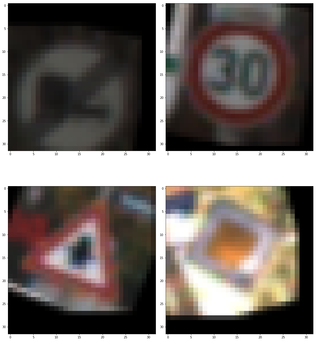
return cv2.warpAffine(img, mat, (w, h))Image below is the Image Augumentation result.

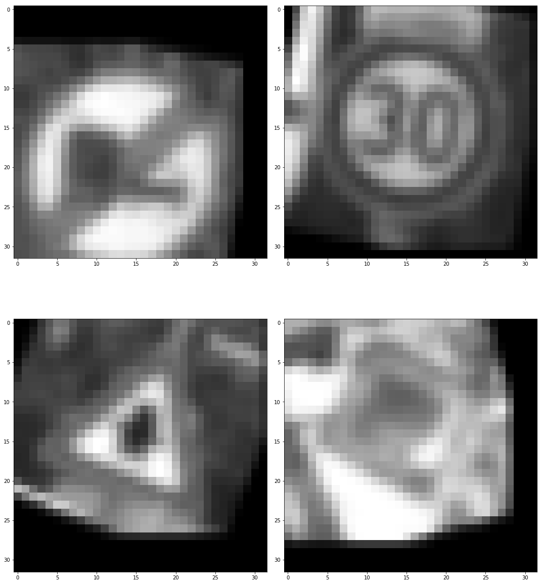
Image below is gray scale of above images

2. Describe how, and identify where in your code, you set up training, validation and testing data. How much data was in each set? Explain what techniques were used to split the data into these sets. (OPTIONAL: As described in the “Stand Out Suggestions” part of the rubric, if you generated additional data for training, describe why you decided to generate additional data, how you generated the data, identify where in your code, and provide example images of the additional data)
since the data set provided a validation data set, thus i do not use data set spliting for validation.
- Number of training examples = 34799
- Number of validation examples = 4410
- Number of testing examples = 12630
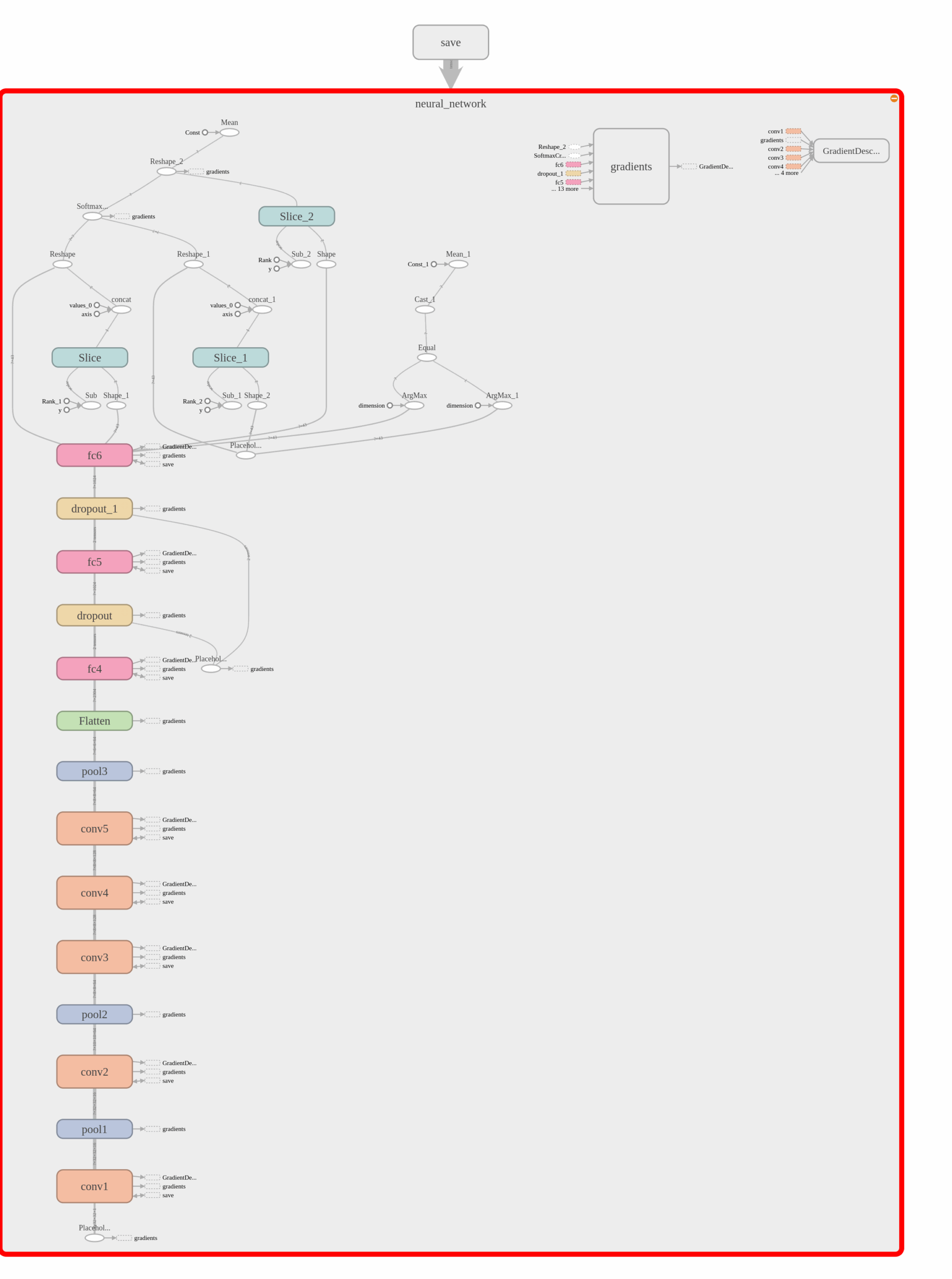
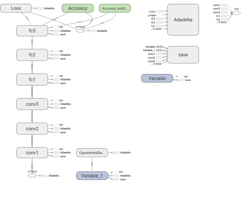
Describe, and identify where in your code, what your final model architecture looks like including model type, layers, layer sizes, connectivity, etc.) Consider including a diagram and/or table describing the final model.
I use a model simliar to AlexNet with smaller number kernel used in conv. layer and less node in hidden layer. It’s because the input size is smaller wiuth this problem.

      ## ini network
      x, y, keep_prob, logits, optimizer, predictions, accuracy = nn()

      # Dro save model
      saver = tf.train.Saver()

      # TensorBoard record
      train_writer = tf.summary.FileWriter("logs/train", sess.graph)

      # Variable initialization
      init = tf.global_variables_initializer()
      sess.run(init)

      # save the acc history
      history = []


      # Record time elapsed for performance check
      last_time = time.time()
      train_start_time = time.time()

      # Run NB_EPOCH epochs of training
      for epoch in range(NB_EPOCH):
          generator = batchGenerator(x_train_processed, y_train_processed)
          while generator.hasNext():
              x_, y_ = generator.next_batch(BATCH_SIZE)
              sess.run(optimizer, feed_dict={x: x_, y: y_, keep_prob: DROPOUT_PROB})

          # Calculate Accuracy Training set
          train_acc = calculate_accuracy(32, accuracy, x, y, x_train_processed, y_train_processed, keep_prob, sess)

          # Calculate Accuracy Validation set
          valid_acc = calculate_accuracy(32, accuracy, x, y, x_valid_processed, y_valid_processed, keep_prob, sess)

          # Record and report train/validation/test accuracies for this epoch
          history.append((train_acc, valid_acc))

          # Print log
          if (epoch+1) % 10 == 0 or epoch == 0 or (epoch+1) == NB_EPOCH:
              print('Epoch %d -- Train acc.: %.4f, valid. acc.: %.4f, used: %.2f sec' %\
                  (epoch+1, train_acc, valid_acc, time.time() - last_time))
              last_time = time.time()

      total_time = time.time() - train_start_time
print('Training time: %.2f sec (%.2f min)' % (total_time, total_time/60))I create a class batchGenerator to manage batch train, which perform batch mangement, it helps the train fucntion cleaner. It also have shuffle function, which randomize the datasets.
- learning rate 0.005
- drop out rate 0.5
- optimizor
- total epochs
- batch size 128
- optimizer: gradient descent algorithm
- Early stop patience 3 # how many epoch will watch for early stop
- Early stop min_delta 0.02 # min. threshold delta change in accuracy
class batchGenerator:
def __init__(self, x, y, shuffle= True):
self.dataX = x
self.dataY = y
self.totalData = len(self.dataX)
if shuffle:
self.shuffle()
def printLog(self):
if len(self.dataX):
print(str(totalData-len(self.dataX))+"https://github.com/"+str(totalData) , end = '\r')
else:
print(str(totalData-len(self.dataX))+"https://github.com/"+str(totalData))
def shuffle(self):
newOrder = np.arange(len(self.dataX))
np.random.shuffle(newOrder)
self.dataX = self.dataX[newOrder]
self.dataY = self.dataY[newOrder]
def hasNext(self):
return len(self.dataX)>0
def next_batch(self,size):
if(len(self.dataX) < size):
size = len(self.dataX)
tempX = self.dataX[0: size]
self.dataX = self.dataX[size:]
tempY = self.dataY[0: size]
self.dataY = self.dataY[size:]
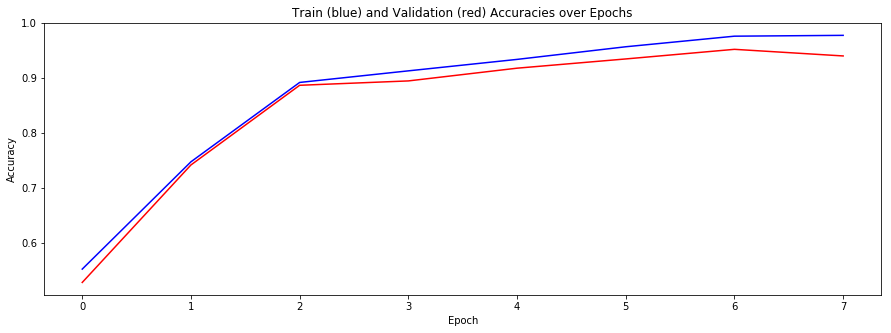
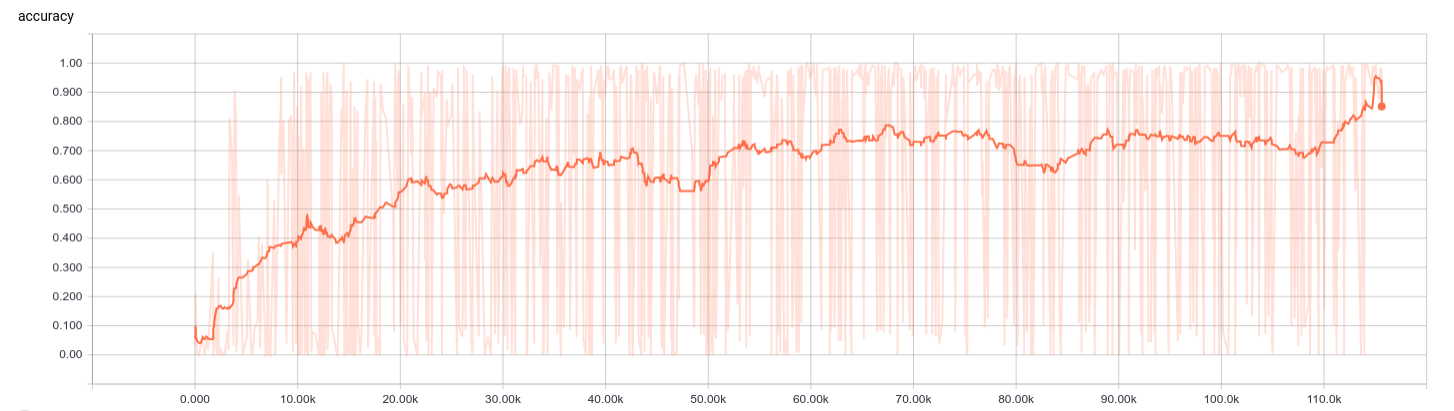
return np.array(tempX), np.array(tempY) The chart above is the accuracy of training and validation during 40 epoch training.
The final model accuracy were:
- training set accuracy of 0.9769
- validation set accuracy of 0.9395
- test set accuracy of 0.9375
The code for calculating the accuracy of the model is located in the the Ipython notebook.
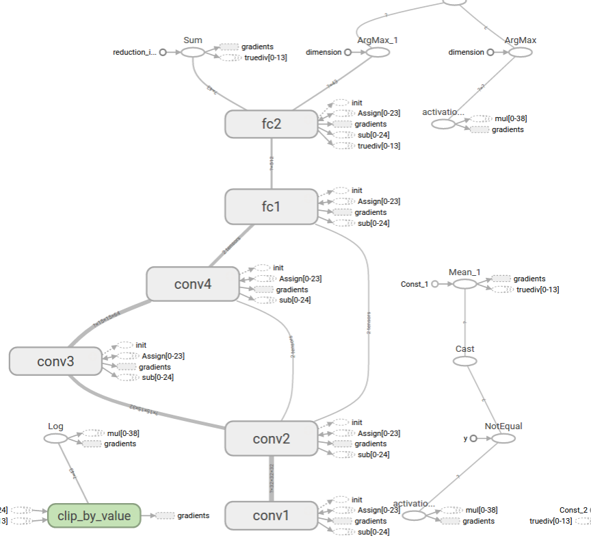
I have try different model.
- Conv 3x3x16 strides 1X1
- Conv 5x5x64 strides 2X2
- Conv 3x3x128 strides 1X1
- Fc 4096
- Fc 1024
- Fc 43 ps no normalization applied


The model need longer time to train to 0.8 acc., which can consider a inefficient model design. The major mistake in this model wasn’t apply batch normalization in the training, which make it need longer to train and do not fully use the nonlinearity of relu.
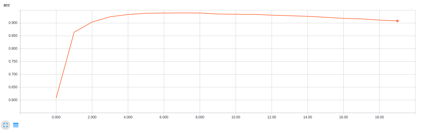
I tried using keras to train the model also.
I use a smaller model, it gave a pretty good result without data augumentation, ~93%.
predict test data 0.933096
code


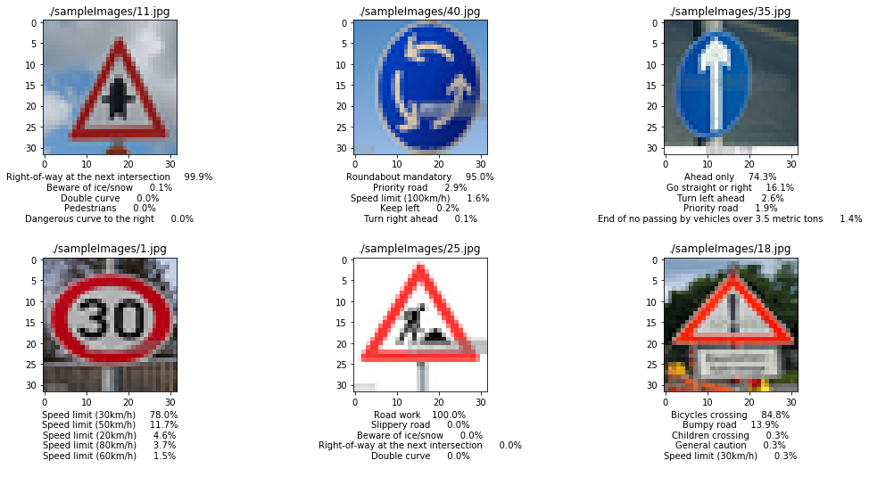
Describe how certain the model is when predicting on each of the five new images by looking at the softmax probabilities for each prediction and identify where in your code softmax probabilities were outputted. Provide the top 5 softmax probabilities for each image along with the sign type of each probability.
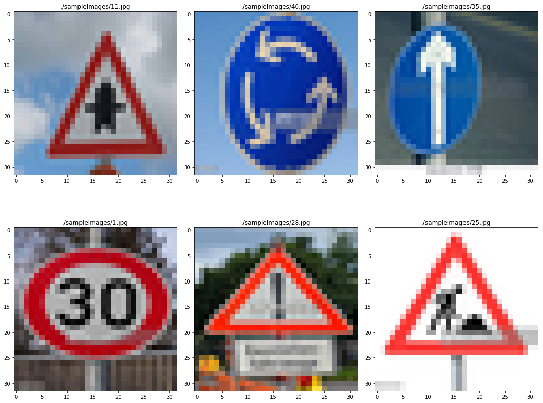
Here are six German traffic signs that I found on the web:

The fifth image much more difficult, it’s because the image not only include single sign, thus it might make model harder to classify into a class.
For others, it have different lighting compare to dataset, they are completly new images, it will be a chanllege to the model.
Here are the results of the prediction:
| Image | Prediction |
|---|---|
| Roundabout mandatory | Roundabout mandatory |
| Ahead only | Ahead only |
| Yield | Yield |
| Speed limit (30km/h) | Speed limit (30km/h) |
| Road work | Road work |
| General caution | Bicycles crossing |
The model was able to correctly guess 5 of the 6 traffic signs, which gives an accuracy of 83.33 %.

For sample image -General caution, it seems predict a completly wrong class.
| class | softmax |
|---|---|
| Bicycles crossing | 84.8% |
| Bumpy Road | 13.9% |
| Children crossing | 0.3% |
| General caution | 0.3% |
| speed limit(30rm/h) | 0.3% |
It seems model do not handle well when image not fully fit with sign. In General caution sample image have a little sign below General caution, it might the reason make model misclassifying it.
For the other sample images, it seems model predit well, all of them have a dominant softmax value over otehr classes.
 https://github.com/hiit-tabata/German-Traffic-Sign-Classification